A New GPU Bundle Adjustment Method for Large-scale Data

大数据的GPU并行区域网平差方法

成果信息

· ZhengM. T., Zhou S. P.*, Zhu J. F. and XiongX. D., (2017). A New GPU Bundle Adjustment Method for Large-scale Data,Photogrammetric Engineering & Remote Sensing, 2017,83(9), 633–641

· https://www.asprs.org/a/publications/pers/2017journals/PERS_09-16_Flipping_Public/HTML/files/assets/basic-html/index.html#43

· 国家自然科学基金青年基金项目(41601502)，中国博士后科学基金项目（2015M572224），中央高校基本科研业务费专项资金资助项目中国地质大学（武汉）杰出人才培育基金（CUG160838,CUG170664）

团队成员

· 郑茂腾，博士，中国地质大学（武汉）信息工程学院，副研究员，主要从事摄影测量与遥感，城市三维建模等方向的研究；

· 周顺平（通讯作者），博士，中国地质大学（武汉）信息工程学院，教授，主要研究方向：GIS理论研究与软件研发，空间数据库与空间分析，GIS软件工程理论与方法.

· 朱俊锋，博士，北京中测智绘科技有限责任公司，总经理，主要从事实景三维建模方向的软件开发与应用工作。

· 熊小东，博士，北京中测智绘科技有限责任公司，总工程师，主要从事摄影测量与遥感，城市三维建模等方向的软件开发与应用工作；

成果介绍

为了进一步解决大数据量带来的平差效率低下的问题，本文引入GPU并行计算技术，同时使用预条件共轭梯度法以及不精确牛顿解法求解区域网平差过程中的法方程，构建了适用于GPU并行计算的全新的区域网平差技术流程. 本方法避免了存储法方程系数矩阵，而是在需要的时候实时的计算该矩阵，使得本算法相较于传统的算法所需的计算机内存空间大幅减少（仅需要存储平差原始数据即可），平差计算速度明显提升，同时计算精度与传统方法相当。初步试验证明，本文的方法在普通电脑上仅需要约1.5分钟即可完成对4500张影像、近900万像点数据的平差计算，且计算精度达到子像素级。

表1 各方法的内存需求对比

Table 1. Memory requirements of different datasets with different schemes(Unit:MB)

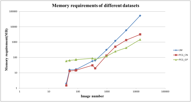
图1 各方法的内存需求对比图

Figure 1. The memory requirements of different schemes with respect to image number

表2 不同数据采用各方法的运行效率对比表格

Table 2. The run time of different datasets with 3 schemes listed in Table 2 (Unit: second)

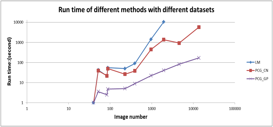
图2 各方法的运行效率对比图

Figure 2. The run time of 4 different schemes with respect to image numbers